Reverse engineering as this article will discuss it is simply the act of figuring out what software that you have no source code for does in a particular feature or function to the degree that you can either modify this code, or reproduce it in another independent work.
In the general sense, ground-up reverse engineering is very hard, and requires several engineers and a good deal of support software just to capture the all of the ideas in a system. However, we’ll find that by using tools available to us, and keeping a good notebook of what’s going on, we should be able to extract the information we need to do what matters: make modifications and hacks to get software that we do not have source code for to do things that it was not originally intended to do.
Why Reverse Engineer?
Answer: Because you can.
It comes down to an issue of power and control. Every computer enthusiast (and essentially any enthusiast in general) is a control-freak. We love the details. We love being able to figure things out. We love to be able to wrap our heads around a system and be able to predict its every move, and more, be able to direct its every move. And if you have source code to the software, this is all fine and good. But unfortunately, this is not always the case.
Furthermore, software that you do not have source code to is usually the most interesting kind of software. Sometimes you may be curious as to how a particular security feature works, or if the copy protection is really “unbreakable”, and sometimes you just want to know how a particular feature is implemented.
It makes you a better programmer
This article will teach you a large amount about how your computer works on a low level, and the better an understanding you have of that, the more efficient programs you can write in general.
[raw] [/raw]
To Learn Assembly Language
If you don’t know assembly language, at the end of this article you will literally know it inside-out. While most first courses and articles on assembly language teach you how to use it as a programming language, you will get to see how to use C as an assembly language generation tool, and how to look at and think about assembly as a C program. This puts you at a tremendous advantage over your peers not only in terms of programming ability, but also in terms of your ability to figure out how the black box works. In short, learning this way will naturally make you a better reverse engineer. Plus, you will have the fine distinction of being able to answer the question “Who taught you assembly language?” with “Why, my C compiler, of course!”
Intro
Compilation in general is split into roughly 5 stages: Preprocessing, Parsing, Translation, Assembling, and Linking.
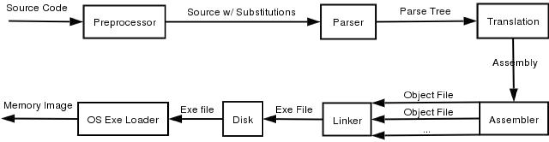
Figure 1. The compilation Process
All 5 stages are implemented by one program in UNIX, namely cc, or in our case, gcc (or g++). The general order of things goes gcc -> gcc -E -> gcc -S -> as -> ld.
Under Microsoft Windows©, however, the process is a bit more obfuscated, but once you delve under the MSVC++ front end, it is essentially the same. Also note that the GNU toolchain is available under Microsoft Windows©, through both the MinGW project as well as the Cygwin Project and behaves the same as under UNIX. Cygwin provides an entire POSIX compatibility layer and UNIX-like environment, where as MinGW just provides the GNU buildchain itself, and allows you to build native windows apps without having to ship an additional dll. Many other commercial compilers exist, but they are omitted for space.
The Compiler
Despite their seemingly disparate approaches to the development environment, both UNIX and Microsoft Windows© do share a common architectural back-end when it comes to compilers (and many many other things, as we will find out in the coming pages). Executable generation is essentially handled end-to-end on both systems by one program: the compiler. Both systems have a single front-end executable that acts as glue for essentially all 5 steps mentioned above.
gcc
gcc is the C compiler of choice for most UNIX. The program gcc itself is actually just a front end that executes various other programs corresponding to each stage in the compilation process. To get it to print out the commands it executes at each step, use gcc -v.
cl.exe
cl.exe is the back end to MSVC++, which is the the most prevalent development environment in use on Microsoft Windows©. You’ll find it has many options that are quite similar to gcc. Try running cl -? for details.
The problem with running cl.exe outside of MSVC++ is that none of your include paths or library paths are set. Running the program vsvars32.bat in the CommonX/Tools directory will give you a shell with all the appropriate environment variables set to compile from the command line. If you’re a fan of Cygwin, you may find it more comfortable to cut and paste vsvars32.bat into cygwin.bat.
The C Preprocessor
The preprocessor is what handles the logic behind all the # directives in C. It runs in a single pass, and essentially is just a substitution engine.
gcc -E
gcc -E runs only the preprocessor stage. This places all include files into your .c file, and also translates all macros into inline C code. You can add -o file to redirect to a file.
cl -E
Likewise, cl -E will also run only the preprocessor stage, printing out the results to standard out.
Parsing And Translation Stages
The parsing and translation stages are the most useful stages of the compiler. Later in this article, we will use this functionality to teach ourselves assembly, and to get a feel for the type of code generated by the compiler under certain circumstances. Unfortunately, the UNIX world and the Microsoft Windows© world diverge on their choice of syntax for assembly, as we shall see in a bit. It is our hope that exposure to both of these syntax methods will increase the flexibility of the reader when moving between the two environments. Note that most of the GNU tools do allow the flexibility to choose Intel syntax, should you wish to just pick one syntax and stick with it. We will cover both, however.
gcc -S
gcc -S will take .c files as input and output .s assembly files in AT&T syntax. If you wish to have Intel syntax, add the option -masm=intel. To gain some association between variables and stack usage, use add -fverbose-asm to the flags.
gcc can be called with various optimization options that can do interesting things to the assembly code output. There are between 4 and 7 general optimization classes that can be specified with a -ON, where 0 <= N <= 6. 0 is no optimization (default), and 6 is usually maximum, although oftentimes no optimizations are done past 4, depending on architecture and gcc version.
There are also several fine-grained assembly options that are specified with the -f flag. The most interesting are -funroll-loops, -finline-functions, and -fomit-frame-pointer. Loop unrolling means to expand a loop out so that there are n copies of the code for n iterations of the loop (ie no jmp statements to the top of the loop). On modern processors, this optimization is negligible. Inlining functions means to effectively convert all functions in a file to macros, and place copies of their code directly in line in the calling function (like the C++ inline keyword). This only applies for functions called in the same C file as their definition. It is also a relatively small optimization. Omitting the frame pointer (aka the base pointer) frees up an extra register for use in your program. If you have more than 4 heavily used local variables, this may be rather large advantage, otherwise it is just a nuisance (and makes debugging much more difficult).
cl -S
Likewise, cl.exe has a -S option that will generate assembly, and also has several optimization options. Unfortunately, cl does not appear to allow optimizations to be controlled to as fine a level as gcc does. The main optimization options that cl offers are predefined ones for either speed or space. A couple of options that are similar to what gcc offers are:
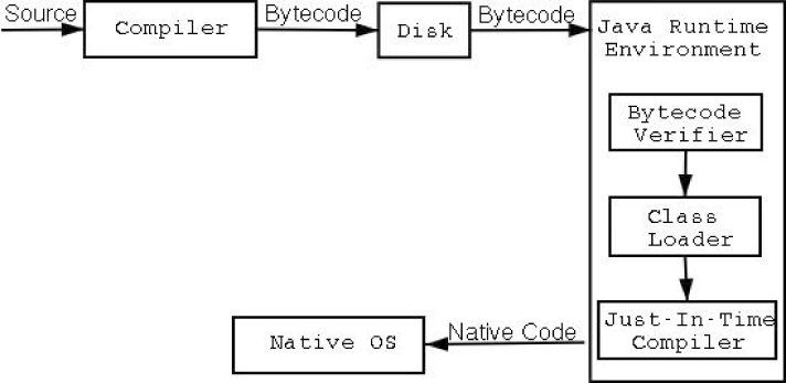
Figure 2. The Java Compile/Execute Path
-Ob<n> – inline functions (-finline-functions)
-Oy – enable frame pointer omission (-fomit-frame-pointer
Assembly Stage
The assembly stage is where assembly code is translated almost directly to machine instructions. Some minimal preprocessing, padding, and instruction reordering can occur, however. We won’t concern ourselves with that too much, as it will become visible during disassembly.
GNU as
as is the GNU assembler. It takes input as an AT&T or Intel syntax asm file and generates a .o object file.
MASM
MASM is the Microsoft© assembler. It is executed by running ml.
Linking Stage
Both Microsoft Windows© and UNIX have similar linking procedures, although the support is slightly different. Both systems support 3 styles of linking, and both implement these in remarkably similar ways.
Static Linking
Static linking means that for each function your program calls, the assembly to that function is actually included in the executable file. Function calls are performed by calling the address of this code directly, the same way that functions of your program are called.
Dynamic Linking
Dynamic linking means that the library exists in only one location on the entire system, and the operating system’s virtual memory system will map that single location into your program’s address space when your program loads. The address at which this map occurs is not always guaranteed, although it will remain constant once the executable has been built. Functions calls are performed by making calls to a compile-time generated section of the executable, called the Procedure Linkage Table, PLT, or jump table, which is essentially a huge array of jump instructions to the proper addresses of the mapped memory.
Runtime Linking
Runtime linking is linking that happens when a program requests a function from a library it was not linked against at compile time. The library is mapped with dlopen() under UNIX, and LoadLibrary() under Microsoft Windows©, both of which return a handle that is then passed to symbol resolution functions (dlsym() and GetProcAddress()), which actually return a function pointer that may be called directly from the program as if it were any normal function. This approach is often used by applications to load user-specified plugin libraries with well-defined initialization functions. Such initialization functions typically report further function addresses to the program that loaded them.
ld/collect2
ld is the GNU linker. It will generate a valid executable file. If you link against shared libraries, you will want to actually use what gcc calls, which is collect2.
link.exe
This is the MSVC++ linker. Normally, you will just pass it options indirectly via cl’s -link option. However, you can use it directly to link object files and .dll files together into an executable. For some reason though, Microsoft Windows© requires that you have a .lib (or a .def) file in addition to your .dlls in order to link against them. The .lib file is only used in the interim stages, but the location to it must be specified on the -LIBPATH: option.
Java Compilation Process
Java is “semi-interpreted” language and it differs from C/C++ and the process described above. What do we mean by “semi-interpreted” language? Java programs execute in the Java Virtual Machine (or JVM), which makes it an interpreted language. On the other hand Java unlike pure interpreted languages passes through an intermediate compilation step. Java code does not compile to native code that the operating system executes on the CPU, rather the result of Java program compilation is intermediate bytecode. This bytecode runs in the virtual machine. Let us take a look at the process through which the source code is turned into executable code and the execution of it.
Java requires each class to be placed in its own source file, named with the same name as the class name and added suffix .java. This basicaly forces any medium sized program to be split in several source files. When compiling source code, each class is placed in its own .class file that contains the bytecode. The java compiler differs from gcc/g++ in the fact that if the class you are compiling is dependent on a class that is not compiled or is modified since it was last compiled, it will compile those additional classes for you. It acts similarly to make, but is nowhere close to it. After compiling all source files, the result will be at least as much class files as the sources, which will combine to form your Java program. This is where the class loader comes into picture along with the bytecode verifier – two unique steps that distinguish Java from languages like C/C++.
The class loader is responsible for loading each class’ bytecode. Java provides developers with the opportunity to write their own class loader, which gives developers great flexibility. One can write a loader that fetches the class from everywhere, even IRC DCC connection. Now let us look at the steps a loader takes to load a class.
When a class is needed by the JVM the loadClass(String name, boolean resolve); method is called passing the class name to be loaded. Once it finds the file that contains the bytecode for the class, it is read into memory and passed to the defineClass. If the class is not found by the loader, it can delegate the loading to a parent class loader or try to use findSystemClass to load the class from local filesystem. The Java Virtual Machine Specification is vague on the subject of when and how the ByteCode verifier is invoked, but by a simple test we can infer that the defineClass performs the bytecode verification. (FIXME maybe show the test). The verifier does four passes over the bytecode to make sure it is safe. After the class is successfully verified, its loading is completed and it is available for use by the runtime.
The nature of the Java bytecode allows people to easily decompile class files to source. In the case where default compilation is performed, even variable and method names are recovered. There are bunch of decompilers out there, but a free one that works well is Jad.
NOW THE FUN BEGINS. THE FIRST STEP IS TO FIGURING OUT WHAT IS GOING ON IN OUR TARGET PROGRAM IS TO GATHER AS MUCH INFORMATION AS WE CAN.SEVERAL TOOLS ALLOW US TO DO THIS ON BOTH PLATFORMS. LET’S TAKE A LOOK AT THEM.
System Wide Process Information
On Microsoft Windows© as on Linux, several applications will give you varying amounts of information about processes running. However, there is a one stop shop for information on both systems.
/proc
The Linux /proc filesystem contains all sorts of interesting information, from where libraries and other sections of the code are mapped, to which files and sockets are open where. The /proc filesystem contains a directory for each currently running process. So, if you started a process whose pid was 1337, you could enter the directory /proc/1337/ to find out almost anything about this currently running process. You can only view process information for processes which you own.
The files in this directory change with each UNIX OS. The interesting ones in Linux are: cmdline – lists the command line parameters passed to the process cwd – a link to the current working directory of the process environ – a list of the environment variables for the process exe – the link to the process executable fd – a list of the file descriptors being used by the process maps – VERY USEFUL. Lists the memory locations in use by this process. These can be viewed directly with gdb to find out various useful things.
Sysinternals Process Explorer
Sysinternals provides an all-around must-have set of utilities. In this case, Process Explorer is the functional equivalent of /proc. It can show you dll mapping information, right down to which functions are at which addresses, as well as process properties, which includes an environment tab, security attributes, what files and objects are open, what the type of objects those handles are for, etc. It will also allow you to modify processes for which you have access to in ways that are not possible in /proc. You can close handles, change permissions, open debug windows, and change process priority.
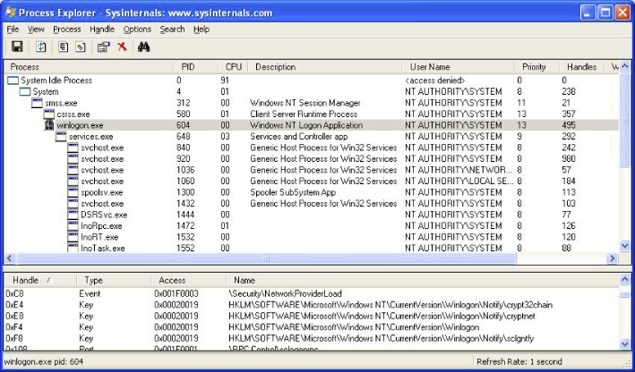
Figure 3. Process Explorer
Obtaining Linking information
The first step towards understanding how a program works is to analyze what libraries it is linked against. This can help us immediately make predictions as to the type of program we’re dealing with and make some insights into its behavior.
ldd
ldd is a basic utility that shows us what libraries a program is linked against, or if its statically linked. It also gives us the addresses that these libraries are mapped into the program’s execution space, which can be handy for following function calls in disassembled output (which we will get to shortly).
depends
depends is a utility that comes with the Microsoft© SDK, as well as with MS Visual Studio. It will show you quite a bit about the linking information for a program. Not only will list dll’s, but it will list which functions in those DLL’s are being imported (used) by the current executable, and how they are imported, and then do this recursively for all dll’s linked against the executable.

Figure 4. Depends
The layout is a little bit much to process at first. When you click on a DLL, you get the functions from this DLL imported by its parent in the tree (upper right, in green). You also get a list of all the functions that this DLL exports. Those that also present in the imports pane are light blue with a dark blue dot. Those that are called somewhere in the entire linked maze are blue, and those that aren’t used at all are grey. Most often all that is used to determine the location of the function is a string and/or an ordinal number, which specifies the numeric index of this function in the export table. Sometimes, the function will be “bound”, which means that the linker took a guess at it’s location in memory and filled it in. Note that bindings may be rejected as “stale”, however, so modifiying this value in the executable won’t always give you the results you suspect.
Obtaining Function Information
The next step in reverse engineering is the ability to differentiate functional blocks in programs. Unfortunately, this can prove to be quite difficult if you aren’t lucky enough to have debug information enabled. We’ll discuss some of those techniques later.
nm
nm lists all of the local and library functions, global variables, and their addresses in the binary. However, it will not work on binaries that have been stripped with strip.
dumpbin.exe
Unfortunately, the closest thing Microsoft Windows© has to nm is dumpbin.exe, which isn’t very great. The only thing it can do is essentially what depends already does: that is list functions used by this binary (dumpbin /imports), and list functions provided by this binary (dumpbin /exports). The only way a binary can export a function (and thus the only way the function is visible) is if that function has the __declspec(dllexport) tag next to it’s prototype.
Luckily, depends is so overkill, it often provides us with more than the information we need to get the job done. Furthermore, the cygwin port of objdump also gets the job done a lot of the time.
Viewing Filesystem Activity
lsof
lsof is a program that lists all open files by the processes running on a system. An open file may be a regular file, a directory, a block special file, a character special file, an executing text reference, a library, a stream or a network file (Internet socket, NFS file or UNIX domain socket). It has plenty of options, but in its default mode it gives an extensive listing of the opened files. lsof does not come installed by default with most of the flavors of Linux/UNIX, so you may need to install it by yourself. On some distributions lsof installs in/usr/sbin which by default is not in your path and you will have to add it. An example output would be:
COMMAND PID USER FD TYPE DEVICE SIZE NODE NAME
bash 101 nasko cwd DIR 3,2 4096 1172699 /home/nasko
bash 101 nasko rtd DIR 3,2 4096 2 /
bash 101 nasko txt REG 3,2 518140 1204132 /bin/bash
bash 101 nasko mem REG 3,2 432647 748736 /lib/ld-2.2.3.so
bash 101 nasko mem REG 3,2 14831 1399832 /lib/libtermcap.so.2.0.8
bash 101 nasko mem REG 3,2 72701 748743 /lib/libdl-2.2.3.so
bash 101 nasko mem REG 3,2 4783716 748741 /lib/libc-2.2.3.so
bash 101 nasko mem REG 3,2 249120 748742 /lib/libnss_compat-2.2.3.so
bash 101 nasko mem REG 3,2 357644 748746 /lib/libnsl-2.2.3.so
bash 101 nasko 0u CHR 4,5 260596 /dev/tty5
bash 101 nasko 1u CHR 4,5 260596 /dev/tty5
bash 101 nasko 2u CHR 4,5 260596 /dev/tty5
bash 101 nasko 255u CHR 4,5 260596 /dev/tty5
screen 379 nasko cwd DIR 3,2 4096 1172699 /home/nasko
screen 379 nasko rtd DIR 3,2 4096 2 /
screen 379 nasko txt REG 3,2 250336 358394 /usr/bin/screen-3.9.9
screen 379 nasko mem REG 3,2 432647 748736 /lib/ld-2.2.3.so
screen 379 nasko mem REG 3,2 357644 748746 /lib/libnsl-2.2.3.so
screen 379 nasko 0r CHR 1,3 260468 /dev/null
screen 379 nasko 1w CHR 1,3 260468 /dev/null
screen 379 nasko 2w CHR 1,3 260468 /dev/null
screen 379 nasko 3r FIFO 3,2 1334324 /home/nasko/.screen/379.pts-6.slack
startx 729 nasko cwd DIR 3,2 4096 1172699 /home/nasko
startx 729 nasko rtd DIR 3,2 4096 2 /
startx 729 nasko txt REG 3,2 518140 1204132 /bin/bash
ksmserver 794 nasko 3u unix 0xc8d36580 346900 socket
ksmserver 794 nasko 4r FIFO 0,6 346902 pipe
ksmserver 794 nasko 5w FIFO 0,6 346902 pipe
ksmserver 794 nasko 6u unix 0xd4c83200 346903 socket
ksmserver 794 nasko 7u unix 0xd4c83540 346905 /tmp/.ICE-unix/794
mozilla-b 5594 nasko 144u sock 0,0 639105 can’t identify protocol
mozilla-b 5594 nasko 146u unix 0xd18ec3e0 639134 socket
mozilla-b 5594 nasko 147u sock 0,0 639135 can’t identify protocol
mozilla-b 5594 nasko 150u unix 0xd18ed420 639151 socket
Here is brief explanation of some of the abbreviations lsof uses in its output:
cwd current working directory
mem memory-mapped file
pd parent directory
rtd root directory
txt program text (code and data)
CHR for a character special file
sock for a socket of unknown domain
unix for a UNIX domain socket
DIR for a directory
FIFO for a FIFO special file
It is pretty handy tool when it comes to investigating program behavior. lsof reveals plenty of information about what the process is doing under the surface.
Fuser | |
A command closely related to lsof is fuser. fuser accepts as a command-line parameter the name of a file or socket. It will return the pid of the process accessing that file or socket. |
Sysinternals Filemon
The analog to lsof in the windows world is the Sysinternals Filemon utility. It can show not only open files, but reads, writes, and status requests as well. Furthermore, you can filter by specific process and operation type. A very useful tool. (FIXME: This has a Linux version as well).
Sysinternals Regmon
The registry in Microsoft Windows© is a key part of the system that contains lots of secrets. In order to try and understand how a program works, one definitely should know how the target interacts with the registry. Does it store configuration information, passwords, any useful information, and so on. Regmon from Sysinternals lets you monitor all or selected registry activity in real time. Definitely a must if you plan to work on any target on Microsoft Windows©.
Viewing Open Network Connections
So this is one of the cases where both Linux and Microsoft Windows© have the same exact name for a utility, and it performs the same exact duty. This utility is netstat.
netstat
netstat is handy little tool that is present on all modern operating systems. It is used to display network connections, routing tables, interface statistics, and more.
How can netstat be useful? Let’s say we are trying to reverse engineer a program that uses some network communication. A quick look at what netstat displays can give us clues where the program connects and after some investigation maybe why it connects to this host. netstat does not only show TCP/IP connections, but also UNIX domain socket connections which are used in interprocess communication in lots of programs. Here is an example output of it:
Listing 1. Netstat output
Active Internet connections (w/o servers)
Proto Recv-Q Send-Q Local Address Foreign Address State
tcp 0 0 slack.localnet:58705 egon:ssh ESTABLISHED
tcp 0 0 slack.localnet:51766 gw.localnet:ssh ESTABLISHED
tcp 0 0 slack.localnet:51765 gw.localnet:ssh ESTABLISHED
tcp 0 0 slack.localnet:38980 clortho:ssh ESTABLISHED
tcp 0 0 slack.localnet:58510 students:ssh ESTABLISHED
Active UNIX domain sockets (w/o servers)
Proto RefCnt Flags Type State I-Node Path
unix 5 [ ] DGRAM 68 /dev/log
unix 3 [ ] STREAM CONNECTED 572608 /tmp/.ICE-unix/794
unix 3 [ ] STREAM CONNECTED 572607
unix 3 [ ] STREAM CONNECTED 572604 /tmp/.X11-unix/X0
unix 3 [ ] STREAM CONNECTED 572603
unix 2 [ ] STREAM 572488
NOTE | |
The output shown is from Linux system. The Microsoft Windows© output is almost identical. |
As you can see there is great deal of info shown by netstat. But what is the meaning of it? The output is divided in two parts – Internet connections and UNIX domain sockets as mentioned above. Here is breifly what the Internet portion of netstat output means. The first column shows the protocol being used (tcp, udp, unix) in the particular connection. Receiving and sending queues for it are displayed in the next two columns, followed by the information identifying the connection – source host and port, destination host and port. The last column of the output shows the state of the connection. Since there are several stages in opening and closing TCP connections, this field was included to show if the connection is ESTABLISHED or in some of the other available states. SYN_SENT, TIME_WAIT, LISTEN are the most often seen ones.
To see complete list of the available states look in the man page for netstat. FIXME: Describe these states.
Depending on the options being passed to netstat, it is possible to display more info. In particular interesting for us is the -p option (not available on all UNIX systems). This will show us the program that uses the connection shown, which may help us determine the behaviour of our target. Another use of this options is in tracking down spyware programs that may be installed on your system. Showing all the network connection and looking for unknown entries is invaluable tool in discovering programs that you are unaware of that send information to the network. This can be combined with the -a option to show all connections. By default listening sockets are not displayed in netstat. Using the -a we force all to be shown. -n shows numerical IP addesses instead of hostnames.
netstat -p as normal user
(Not all processes could be identified, non-owned process info
will not be shown, you would have to be root to see it all.)
Active Internet connections (w/o servers)
Proto Recv-Q Send-Q Local Address Foreign Address State PID/Program name
tcp 0 0 slack.localnet:58705 egon:ssh ESTABLISHED -
tcp 0 0 slack.localnet:58766 winston:www ESTABLISHED 5587/mozilla-bin
netstat -npa as root user
Active Internet connections (servers and established)
Proto Recv-Q Send-Q Local Address Foreign Address State PID/Program name
tcp 0 0 0.0.0.0:139 0.0.0.0:* LISTEN 390/smbd
tcp 0 0 0.0.0.0:6000 0.0.0.0:* LISTEN 737/X
tcp 0 0 0.0.0.0:22 0.0.0.0:* LISTEN 78/sshd
tcp 0 0 10.0.0.3:58705 128.174.252.100:22 ESTABLISHED 13761/ssh
tcp 0 0 10.0.0.3:51766 10.0.0.1:22 ESTABLISHED 897/ssh
tcp 0 0 10.0.0.3:51765 10.0.0.1:22 ESTABLISHED 896/ssh
tcp 0 0 10.0.0.3:38980 128.174.252.105:22 ESTABLISHED 8272/ssh
tcp 0 0 10.0.0.3:58510 128.174.5.39:22 ESTABLISHED 13716/ssh
So this output shows that mozilla has established a connection with winston for HTTP traffic (since port is www(80)). In the second output we see that the SMB daemon, X server, and ssh daemon listen for incoming connections.
Gathering Network Data
Collecting network data is usually done with a program called sniffer. What the program does is to put your ethernet card into promiscuous mode and gather all the information that it sees. What is a promiscuous mode? Ethernet is a broadcast media. All computers broadcast their messages on the wire and anyone can see those messages. Each network interface card (NIC), as a hardcoded physical address called MAC (Media Access Control) address, which is used in the Ethernet protocol. When sending data over the wire, the OS specifies the destination of the data and only the NIC with the destination MAC address will actually process the data. All other NICs will disregard the data coming on the wire. When in promiscuous mode, the card picks up all the data that it sees and sends it to the OS. In this case you can see all the data that is flowing on your local network segment.
Disclaimer | |
Switched networks eliminate the broadcast to all machines, but sniffing traffic is still possible using certain techniques like ARP poisoning. (FIXME: link with section on ARP poisoning if we have one.) |
Several popular sniffing programs exist, which differ in user interface and capabilities, but any one of them will do the job. Here are some good tools that we use on a daily basis:
• ethereal – one of the best sniffers out there. It has a graphical interface built with the GTK library. It is not just a sniffer, but also a protocol analyzer. It breaks down the captured data into pieces, showing the meaning of each piece (for example TCP flags like SYN or ACK, or even kerberos or NTLM headers). Furthermore, it has excellent packet filtering mechanisms, and can save captures of network traffic that match a filter for later analysis. It is available for both Microsoft Windows© and Linux and requires (as almost any sniffer) the pcap library. Ethereal is available at www.ethereal.com and you will need libpcap for Linux orWinPcap for Microsoft Windows©.
• tcpdump – one of the first sniffing programs. It is a console application that prints info to the screen. The advantage is that it comes by default with most Linux distributions. Microsoft Windows© version is available as well, called WinDump.
• ettercap – also a console based sniffer. Uses the ncurses library to provide console GUI. It has built in ARP poisoning capability and supports plugins, which give you the power to modify data on the fly. This makes it very suitable for all kinds of Man-In-The-Middle attacks (MITM), which will we will describe in chapter (FIXME: link). Ettercap isn’t that great a sniffer, but nothing prevents you from using its ARP poisoning and plugin features while also running a more powerful sniffer such as ethereal.
Now that you know what a sniffer is and hopefully learned how to use basic functionality of your favorite one, you are all set to gather network data. Let’s say you want to know how does a mail client authenticate and fetch messages from the server. Since the protocol in use is POP3, we should instruct ethereal (our sniffer of choice) to capture traffic only destined to port 110 or originating from port 110. In our case since we want to capture both directions of the traffic we can set the filter to be tcp.port == 110. If you have a lot of machines checking mail at the same time on a network with a hub, you might want to restrict the matching only to your machine and the server you are connecting to. Here is an example of captured packet in ethereal:
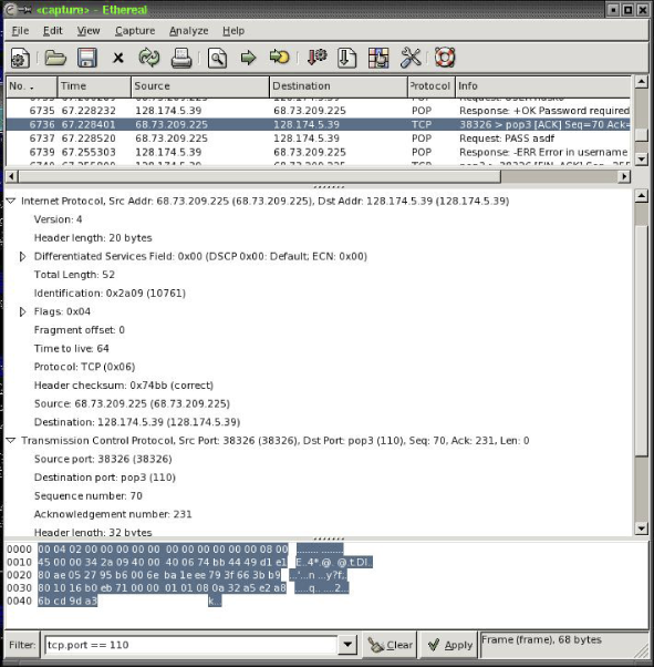
Figure 5. Ethereal capture
Ethereal breaks down the packet for us, showing what each part of the data means. For example, it shows that the Internet Protocol version is 4 or that the header checksum is 0x74bb and is in fact the correct checksum for that packet. It shows in similar manner details for each part of the header and the data at the end of the packet if any.
Using packet captures, one can trace the flow of a protocol to better understand how an application works, or even try to reverse engineer the protocol itself if unknown.
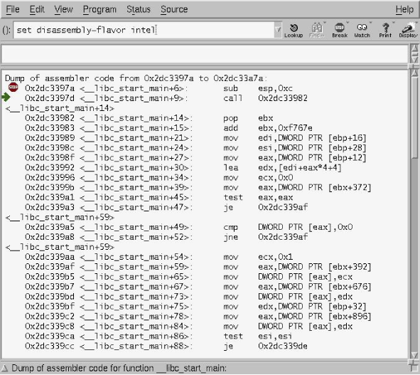
Figure 6. ASM in DDD
Determining Program Behavior
There are a couple of tools that allow us to look into program behavior at a more closer level. Lets look at some of these:
Tracing System Calls
This section is really only relevant for to our efforts under UNIX, as Microsoft Windows© system calls change regularly from version to version, and have unpredictable entry points.
strace/truss(Solaris)
These programs trace system calls a program makes as it makes them.
Useful options:
-f (follow fork)
-ffo filename (output trace to filename.pid for forking)
-i (Print instruction pointer for each system call)
Tracing Library Calls
Now we’re starting to get to the more interesting stuff. Tracing library calls is a very powerful method of system analysis. It can give us a *lot* of information about our target.
ltrace
This utility is extremely useful. It traces ALL library calls made by a program.
Useful options:
-S (display syscalls too)
-f (follow fork)
-o filename (output trace to filename)
-C (demangle C++ function call names)
-n 2 (indent each nested call 2 spaces)
-i (prints instruction pointer of caller)
-p pid (attaches to specified pid)
API Monitor
API Monitor is incredible. It will let you watch .dll calls in real time, filter on type of dll call, view.
HERE I AM SKIPPING A FEW THINGS, CAUSE I DON’T CONSIDER THEM TO BE IMPORTANT PLUS THIS WILL ONLY LENGTHEN THE ARTICLE
User-level Debugging
DDD
DDD is the Data Display Debugger, and is a nice GUI front-end to gdb, the GNU debugger. For a long time, the authors believed that the only thing you really needed to debug was gdb at the command line. However, when reverse engineering, the ability to keep multiple windows open with stack contents, register values, and disassembly all on the same workspace is just too valuable to pass up.
Also, DDD provides you with a gdb command line window, and so you really aren’t missing anything by using it. Knowing gdb commands is useful for doing things that the UI is too clumsy to do quickly. gdb has a nice built-in help system organized by topic. Typing help will show you the categories. Also, DDD will update the gdb window with commands that you select from the GUI, enabling you to use the GUI to help you learn the gdb command line. The main commands we will be interested in are run, break, cont, stepi, nexti, finish, disassemble, bt, info [registers/frame], and x. Every command in gdb can be followed by a number N, which means repeat N times. For example, stepi 1000 will step over 1000 assembly instructions.
Setting Breakpoints
A breakpoint stops execution at a particular location. Breakpoints are set with the break command, which can take a function name, a filename:line_number, or *0xaddress. For example, to set a breakpoint at the aforementioned __libc_start_main(), simply specify break __libc_start_main. In fact, gdb even has tab completion, which will allow you to tab through all the symbols that start with a particular string (which, if you are dealing with a production binary, sadly won’t be many).
Viewing Assembly
Ok, so now that we’ve got a breakpoint set somewhere, (let’s say __libc_start_main). To view the assembly in DDD, go to the View menu and select source window. As soon as we enter a function, the disassembly will be shown in the bottom half of the source window. To change the syntax to the more familar Intel variety, go to Edit->Gdb Settings… under Disassembly flavor. This can also be accomplished with set disassembly-flavor intel from the gdb prompt. But using the DDD menus will save your settings for future sessions.
Viewing Memory and the Stack
In gdb, we can easily view the stack by using the x command. x stands for Examine Memory, and takes the syntax x /<Number><format letter><size letter> <ADDRESS>. Format letters are (octal), x(hex), d(decimal), u(unsigned decimal), t(binary), f(float), a(address), i(instruction), c(char) and s(string). Size letters are b(byte), h(halfword), w(word), g(giant, 8 bytes). For example, x /32xw 0x400000 will dump 32 words (32 bit integers) starting at 0×400000. Note that you can also use registers in place of the address, if you prefix them with a $. For example, x /32xw $esp will view the top 32 words on the stack.
DDD has some nice capabilities for viewing arbitrary dumps of memory relating to the registers. Go to View->Data Window… Once the Data Window is open, go to Display (hold down the mouse button as you click), and go to Other.. You can type in any symbol, variable, expression, or gdb command (in backticks) in this window, and it will be updated every time you issue a command to the debugger. A couple good ones to do would be x /32xw $esp and x/16sb $esp. Click the little radio button to add these to the menu, and you can then open the stack from this display and it will be updated in real time as you step through your program.
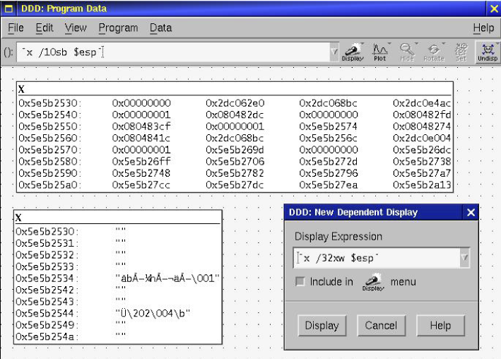
Figure 7. Stack Displays with New Display Window
Viewing Memory as Specific Data Structures
So DDD has fantastic ability to lay out data structures graphically, also trough the Display window mentioned above. Simply cast a memory address to a pointer of a particular type, and DDD will plot the structure in its graph window. If the data structure contains any pointers, you can click on these and DDD will open up a display for that structure as well.
Oftentimes, programs we’re interested in won’t have any debugging symbols, and as such, we won’t be able to view any structures in an easy to understand form. For seldom used structures, this isn’t that big of a deal, as you can just take them apart using the x command. However, if you are dealing with more complicated data structures, you may want to have a set of types available to use again and again. Luckily, through the magic of the ELF format, this is relatively easy to achieve. Simply define whatever structures or classes you suspect are used and include whatever headers you require in a .c file, and then compile it with gcc -shared. This will produce a .so file. Then, from within gdb but before you begin debugging, run the command set env LD_PRELOAD=file.so. From then on, you will be able to use these types in that gdb/DDD session as if they were compiled in to the program itself. (FIXME: Come up with a good example for this).
Using watchpoints
-> Example using gdb to set breakpoints in functions with and without debugging symbols.
-> FIXME: Test watchpoints
WinDbg
WinDbg is part of the standart Debugging Tools for Microsoft Windows© that everyone can download for free from. Microsoft© offers few different debuggers, which use common commands for most operations and ofcourse there are cases where they differ. Since WinDbg is a GUI program, all operations are supposed to be done using the provided visual components. There is also a command line embeded in the debugger, which lets you type commands just like if you were to use a console debugger like ntsd. The following section briefly mentions what commands are used to do common everyday tasks. For more complete documentation check the Help file that comes with WinDbg. An example debugging session is presented to help clarify the usage of the most common commands.
Breakpoints
Breakpoints can be set, unset, or listed with the GUI by using Edit->Breakpoints or the shortcut keys Alt+F9. From the command line one can set breakpoints using the bp command, list them using bl command, and delete them using bc command. One can set breakpoints both on function names (provided the symbol files are available) or on a memory address. Also if source file is available the debugger will let you set breakpoints on specific lines using the format bX filename:linenumber.
Viewing Assembly
In WinDbg you can use View->Disassembly option to open a window which will show you the disassembly of the current context. In ntsd you can use the u to view the disassembled code.
Stack operations
There are couple of things one usually does with the stack. One is to view the frames on the stack, so it can be determined which function called which one and what is the current context. This is done using the k command and its variations. The other common operation is to view the elements on the stack that are part of the current stack frame. The easiest way to do so is using db esp ebp, but it has its limitations. It assumes that the %ebp register actually points to the begining of the stack frame. This is not always true, since omission of the frame pointer is common optimization technique. If this is the case, you can always see what the %esp register is pointing to and start examining memory from that address. The debugger also allows you to “walk” the stack. You can move to any stack frame using .frame X where X is the number of the frame. You can easily get the frame numbers using kn. Keep in mind that the frames are counted starting from 0 at the frame on top of the stack.
Reading and Writing to Memory
Reading memory is accomplished with the d* commands. Depending on how you want to view the data you use a specific variation of this command. For example to see the address to which a pointer is pointing, we can use dp or to view the value of a word, one can use dw. The help file says that one can view memory using ranges, but one can also use lengths to make it easy to display memory. For example if we want to see 0×10 bytes at memory location 0x77f75a58 you can either say db 77f75a58 77f75a58+10 or less typing gives you db 77f75a58 l 10.
Provided that you have symbols/source files, the dt is very helpful. It tries to find the data type of the sybol or memory location and display it accordingly.
Tips and tricks
Knowing your debugger can save you lots of time and pain in debugging either your own programs or when reverse engineering other’s. Here are few things we find useful and time saving. This is not a complete list at all. If you know other tricks and want to contribute, let us know. poi() – this command dereferences a pointer to give you the value that it is pointing to. Using this with user-defined aliases gives you convinient way of viewing data.
Example
Let’s set a breakpoint in on the function main
0:000> bp main
*** WARNING: Unable to verify checksum for test.exe
Let’s set a breakpoint in on the function main
0:000> g
Breakpoint 0 hit
eax=003212e8 ebx=7ffdf000 ecx=00000001 edx=7ffe0304 esi=00000a28 edi=00000000
eip=00401010 esp=0012fee8 ebp=0012ffc0 iopl=0 nv up ei pl zr na po nc
cs=001b ss=0023 ds=0023 es=0023 fs=0038 gs=0000 efl=00000246
test!main:
00401010 55 push ebp
Enable loading of line information if available
0:000> .lines
*** ERROR: Symbol file could not be found. Defaulted to export symbols for ntdll.dll –
Line number information will be loaded
Set the stepping to be by source lines
0:000> l+t
Source options are 1:
1/t – Step/trace by source line
Enable displaying of source line
0:000> l+s
Source options are 5:
1/t – Step/trace by source line
4/s – List source code at prompt
Start stepping through the program
0:000> p
*** WARNING: Unable to verify checksum for test.exe
eax=003212e8 ebx=7ffdf000 ecx=00000001 edx=7ffe0304 esi=00000a28 edi=00000000
eip=00401016 esp=0012fed4 ebp=0012fee4 iopl=0 nv up ei pl nz na po nc
cs=001b ss=0023 ds=0023 es=0023 fs=0038 gs=0000 efl=00000206
> 6: char array [] = { ‘r’, ‘e’, ‘v’, ‘e’, ‘n’, ‘g’ };
test!main+6:
00401016 c645f072 mov byte ptr [ebp-0x10],0×72 ss:0023:0012fed4=05
0:000>
eax=003212e8 ebx=7ffdf000 ecx=00000001 edx=7ffe0304 esi=00000a28 edi=00000000
eip=0040102e esp=0012fed4 ebp=0012fee4 iopl=0 nv up ei pl nz na po nc
cs=001b ss=0023 ds=0023 es=0023 fs=0038 gs=0000 efl=00000206
> 7: int intval = 123456;
test!main+1e:
0040102e c745fc40e20100 mov dword ptr [ebp-0x4],0x1e240 ss:0023:0012fee0=0012ffc0
0:000>
eax=003212e8 ebx=7ffdf000 ecx=00000001 edx=7ffe0304 esi=00000a28 edi=00000000
eip=00401035 esp=0012fed4 ebp=0012fee4 iopl=0 nv up ei pl nz na po nc
cs=001b ss=0023 ds=0023 es=0023 fs=0038 gs=0000 efl=00000206
> 9: test = (char*) malloc(strlen(“Test”)+1);
test!main+25:
00401035 6840cb4000 push 0x40cb40
0:000>
eax=00321018 ebx=7ffdf000 ecx=00000000 edx=00000005 esi=00000a28 edi=00000000
eip=00401051 esp=0012fed4 ebp=0012fee4 iopl=0 nv up ei pl nz na po nc
cs=001b ss=0023 ds=0023 es=0023 fs=0038 gs=0000 efl=00000206
> 10: if (test == NULL) {
test!main+41:
00401051 837df800 cmp dword ptr [ebp-0x8],0×0 ss:0023:0012fedc=00321018
0:000>
eax=00321018 ebx=7ffdf000 ecx=00000000 edx=00000005 esi=00000a28 edi=00000000
eip=00401061 esp=0012fed4 ebp=0012fee4 iopl=0 nv up ei pl nz na po nc
cs=001b ss=0023 ds=0023 es=0023 fs=0038 gs=0000 efl=00000206
> 13: strncpy(test, “Test”, strlen(“Test”));
test!main+51:
00401061 6848cb4000 push 0x40cb48
0:000>
eax=00321018 ebx=7ffdf000 ecx=00000000 edx=74736554 esi=00000a28 edi=00000000
eip=00401080 esp=0012fed4 ebp=0012fee4 iopl=0 nv up ei pl nz ac po nc
cs=001b ss=0023 ds=0023 es=0023 fs=0038 gs=0000 efl=00000216
> 14: test[4] = 0×00;
test!main+70:
00401080 8b4df8 mov ecx,[ebp-0x8] ss:0023:0012fedc=00321018
0:000>
eax=00321018 ebx=7ffdf000 ecx=00321018 edx=74736554 esi=00000a28 edi=00000000
eip=00401087 esp=0012fed4 ebp=0012fee4 iopl=0 nv up ei pl nz ac po nc
cs=001b ss=0023 ds=0023 es=0023 fs=0038 gs=0000 efl=00000216
> 16: printf(“Hello RevEng-er, this is %sn”, test);
test!main+77:
00401087 8b55f8 mov edx,[ebp-0x8] ss:0023:0012fedc=00321018
Display the array as bytes and ascii
0:000> db array array+5
0012fed4 72 65 76 65 6e 67 reveng
View the type and value of intval
0:000> dt intval
Local var @ 0x12fee0 Type int
123456
View the type and value of test
0:000> dt test
Local var @ 0x12fedc Type char*
0×00321018 “Test”
View the memory test points to manually
0:000> db 00321018 00321018+4
00321018 54 65 73 74 00 Test.
Quit the debugger
0:000> q
quit:
Unloading dbghelp extension DLL
Unloading exts extension DLL
Unloading ntsdexts extension DLL
THINGS I’D BE LEAVING IN THIS ARTICLE
• Executable formats
• Code Modification
• Network Application Interception
LOOK OUT FOR 2ND ARTICLE OF THIS SERIES FOR ALL THESE.
No comments:
Post a Comment